Designing a Telemetry Pipeline That Scales [Part 1]: Architecture, Agents, and Forwarders
Why observability pipelines fail at 100 to 1,000 servers, and how to redesign collection and processing with OpenTelemetry.
This is Part 1 of a two-part series on building a telemetry pipeline for 1,000 servers. In this part, we focus on the collection path: where common designs break, how to split the system into clear tiers, and why agents and forwarders should have very different jobs.
We started with a setup that worked well for the first year: VictoriaMetrics’ vmagent instead of Prometheus for metrics collection, and Jaeger with Cassandra for distributed traces. At 100 to 150 servers, everything ran smoothly. vmagent handled cardinality and write load much better than traditional Prometheus, so we felt good about the metrics side.
Then we doubled the fleet to 300 servers, and doubled again to 600.
vmagent held up well. Jaeger did not. Cassandra started to struggle under the load of billions of trace spans. The OTel collectors on each app server were using 2-3+ GB of RAM each because they were doing too much: relabeling, sampling, batching, and other work that should not run on the same machine as a production database.
We needed a different design. Not “add more agents” or “tune Jaeger,” but a design where each layer has one clear job and does not interfere with the others.
This post explains the architecture we used to handle metrics and traces across 100 to 1,000+ servers.
1. The Problem: What Breaks When You Scale Naively#
Telemetry pipelines almost always start simple and become more complex over time. The problem is that the common mid-scale designs often share the same flaws: no proper buffer, poor sampling, and tight coupling between collection and storage. Here are three common patterns and what breaks in each one.
Pattern 1: Agents Write Directly to Storage (Small Teams, Early Stage)#
The starting point for most teams:
┌──────────────────────────────────────────────────────────────┐
│  App / DB Server                                             │
│                                                              │
│  ┌─────────────────────────────────────────────────────┐    │
│  │  OTel Collector (agent mode)                        │    │
│  │  - hostmetrics, docker_stats, DB receivers          │    │
│  │  - filter, relabel, attribute enrichment            │    │
│  │  - probabilistic head sampling for traces           │    │
│  │  - batch + compression                              │    │
│  └──────────────────────┬──────────────────────────────┘    │
│                         │                                    │
└─────────────────────────┼────────────────────────────────────┘
                          │ remote_write / OTLP
                          ▼
              ┌───────────────────────────────┐
              │  vmagent → VictoriaMetrics    │  (metrics)
              │  Jaeger Collector → Cassandra │  (traces)
              └───────────────────────────────┘
This works at 10 to 50 servers. At 300 and beyond, three things break simultaneously:
Agents are doing too much on production machines. When the agent is filtering, relabeling, enriching attributes, and head-sampling traces on top of scraping six or more sources, it competes with your application for CPU. A PostgreSQL primary does not care that your collector is batching 10,000 spans. It only sees latency spikes.
Head sampling loses the traces we need. With probabilistic head sampling at the agent, we decide to keep or drop a trace before the request finishes. An error trace that took 3 seconds has the same 5% chance of being kept as a fast, healthy trace. During incidents, we often lose the traces we need most.
Jaeger’s Cassandra backend becomes expensive to run at scale. Cassandra is a capable database, but running it at the write volume needed for billions of trace spans per day becomes its own infrastructure project. As span volume grows, we spend more time tuning compaction, adding nodes, and managing repair cycles. The trace storage layer starts to need its own team.
Pattern 2: Per-Fleet Forwarder Pairs (Mid-Scale, Common in Practice)#
Teams that outgrow Pattern 1 typically reach for per-fleet forwarding. The instinct is reasonable: split the fleet into logical groups (web tier, DB tier, Kafka tier) and give each group its own pair of forwarders for redundancy.
Web Fleet (200 servers):
  Agent ─┐
  Agent ─┤→ [ Forwarder-A ]─┐
  Agent ─┘  [ Forwarder-B ]─┤──→ VictoriaMetrics
                             │         +
DB Fleet (50 servers):       │    Jaeger (Cassandra)
  Agent ─┐                   │
  Agent ─┤→ [ Forwarder-C ]─┤
  Agent ─┘  [ Forwarder-D ]─┘

Kafka Fleet (18 brokers):
  Agent ─┐
  Agent ─┤→ [ Forwarder-E ]───→ VictoriaMetrics
  Agent ─┘  [ Forwarder-F ]
This solves the single-agent-does-everything problem. Processing moves off app servers. Each fleet pair provides some redundancy. Many companies run exactly this design.
Here is what still fails:
Tail sampling cannot work correctly with ordinary load balancing. Sending traces to forwarders is not the problem by itself. The problem is that, in a per-fleet forwarder pair, a normal load balancer can send Span 1 of a trace to Forwarder-A and Span 2 to Forwarder-B. Neither instance sees the full trace, so tail sampling cannot work. We are still stuck with head sampling and still lose error traces at random.
No buffer between forwarders and storage. When VictoriaMetrics is being upgraded or Cassandra is busy with compaction, every forwarder has nowhere to queue data. We can add disk queues to each forwarder, but then we have to size those queues separately for each fleet, and we still do not get a reliable replay path if the forwarder itself restarts.
Cardinality control is fragmented. Using forwarders for filtering and transforms is not the problem. The problem is having a separate forwarder pair for each fleet. Each pair ends up with its own copy of the rules, so there is no single place to enforce cardinality policy across the whole system. When a new deployment introduces a high-cardinality label, we have to update every forwarder pair separately.
Scaling is operationally complex. When the web fleet grows from 200 to 500 servers, we have to scale Forwarder-A and Forwarder-B separately from the DB fleet. We end up with different instance counts, different memory settings, and different alert thresholds for each forwarder group. The operational overhead grows with the number of fleet groups, not with the total number of servers.
Jaeger’s Cassandra is still the bottleneck. Moving processing to forwarders does not change the trace storage problem. Cassandra still receives the full span volume from all forwarder pairs.
Pattern 3: Shared Forwarder Pool Without a Buffer (Close, but Not Quite)#
Some teams consolidate the per-fleet forwarder pairs into a single shared pool:
All Agents → Load Balancer → [ Forwarder Pool: 4-6 instances ] → VictoriaMetrics
                                                               → Jaeger / Tempo
This fixes the operational fragmentation. One forwarder pool, one set of configs, one scaling unit. Closer to the right design.
The remaining problems:
Still no shared buffer or backpressure layer between forwarders and storage. A VictoriaMetrics rolling upgrade creates a gap in metrics. A Tempo or Jaeger outage drops traces. Each forwarder has to manage its own disk queue, there is no shared replay window, and backpressure is still handled locally on each instance instead of being absorbed by a shared durable layer like Kafka.
Tail sampling still requires special routing. A shared pool of forwarders solves the management problem, but it does not solve trace affinity by itself. With 4 to 6 forwarders behind a standard load balancer, spans from the same trace can still split across instances. Tail sampling only works when every span of a trace reaches the same forwarder, so the load balancer must use consistent hashing on trace ID. Many teams stop at a shared pool, skip that routing step, and then find that tail sampling is unreliable and fall back to head sampling.
What the Right Architecture Has to Guarantee#
The patterns above point to five requirements that the final design must satisfy:
- Agents must be lightweight. All processing must happen on machines dedicated to processing.
- No single points of failure at any tier, including the forwarder pool.
- Tail sampling must work reliably, which requires consistent trace ID routing to the same forwarder instance and enough memory per instance to buffer a full 30-second trace window.
- Every tier must keep accepting data when its downstream is unavailable, queue it safely, and replay it automatically when the downstream recovers. This means a shared Kafka buffer, not per-forwarder disk queues.
- Storage must be fully decoupled from the collection rate. A slow storage write must not back-pressure the forwarder, the agents, or the applications running on those servers.
The four-tier design in the next sections satisfies all five. The key addition over Pattern 3 is Kafka as a shared, durable buffer between the forwarder pool and storage, plus consistent trace ID routing at the load balancer.
2. Scope: What We Handle and Why#
Signals: Metrics and Traces Only#
This pipeline handles metrics and traces. Logs are intentionally excluded.
Metrics and traces fit the same overall architecture well: lightweight agents on servers, centralized processing at the forwarder tier, durable buffering in Kafka, and separate storage backends sized for each signal. They differ in format and query patterns, but they both benefit from the same core design principles: decoupled ingestion, controlled processing, and replay during downstream failures.
Logs are different. Log volume is usually much higher, retention rules are different, and the query model is different as well. In practice, logs need their own pipeline, their own controls, and usually their own storage backend, such as Loki or VictoriaLogs. Mixing logs into the same collector pipeline makes tuning harder and increases the blast radius when one signal spikes.
Why Grafana Tempo Instead of Jaeger#
The previous setup used Jaeger, and it is a reasonable place to start. The main issue at scale is the storage model.
Jaeger can use Cassandra, Elasticsearch, or OpenSearch as storage backends, but that still leaves us operating and scaling a dedicated trace storage system. At high span volume, that backend becomes a major part of the tracing stack, with its own scaling, tuning, and operational cost.
Grafana Tempo fits this design better because it stores traces directly in object storage such as S3, GCS, or MinIO. There is no separate hot trace database to manage. That keeps the storage layer simpler, scales more naturally with trace volume, and fits well with a Kafka-buffered pipeline where processing and storage are already decoupled.
The migration path is also simple. Tempo accepts OTLP natively, and the OTel Collector can forward legacy Jaeger traffic during the transition.
What Each Server Runs#
The fleet is not uniform. Each server runs the base receivers (hostmetrics + otlp) plus service-specific receivers for whatever it hosts. k8s_cluster runs once per cluster on a dedicated collector, not on each worker node.
| Server Type | Receivers |
|---|---|
| Bare metal PostgreSQL primary | hostmetrics, otlp, postgresql |
| Monolithic app server (systemd) | hostmetrics, otlp |
| Docker app server | hostmetrics, docker_stats, otlp |
| Docker + Redis | hostmetrics, docker_stats, otlp, redis |
| Kafka broker (Docker) | hostmetrics, docker_stats, otlp, kafkametrics |
| Kubernetes worker node | hostmetrics, kubeletstats, otlp |
The full receiver list for databases, caches, brokers, and web servers is in the opentelemetry-collector-contrib receiver directory. The companion repository has pre-built profiles for the most common server types.
3. The Numbers: Making the Math Concrete#
“Millions of events per second” is the scale this architecture targets. The exact number depends on the fleet mix. A real enterprise fleet usually includes Kubernetes worker nodes, plain Linux VMs, databases, middleware, and some Docker hosts, along with instrumented application services.
Metrics Volume#
Series count depends on the server role. Not every receiver runs on every server, and not every server emits the same amount of telemetry.
Profile A — Docker app server:

  hostmetrics    (CPU × cores, memory, disk × partitions, network × NICs)    ~1,200 series
  docker_stats   (100 containers × ~80 series — per-core, per-NIC, per-device) ~8,000 series
  app metrics    (custom OTel instrumentation via otlp)                       ~2,000 series
  DB + middleware (postgresql, redis, nginx combined)                            ~800 series
  ─────────────────────────────────────────────────────────────────────────────────────────
  Total                                                                       ~12,000 series

Profile B — Kubernetes worker node:

  hostmetrics    (same as above)                                              ~1,200 series
  kubeletstats   (50 pods/node × ~30 series — actual cpu, memory, network)   ~1,500 series
  app metrics    (spans and custom metrics via otlp)                          ~2,000 series
  DB + middleware (if services run on the node)                                 ~800 series
  ─────────────────────────────────────────────────────────────────────────────────────────
  Total                                                                        ~5,500 series

Profile C — Linux VM / DB / middleware node:

  hostmetrics    (same as above)                                              ~1,200 series
  service metrics (postgresql, mysql, redis, kafka, nginx, rabbitmq, etc.)   ~1,500 to 4,000 series
  app metrics    (if the node also runs an instrumented service)              ~500 to 1,500 series
  ─────────────────────────────────────────────────────────────────────────────────────────
  Total                                                                        ~3,000 to 6,000 series

k8s_cluster (1 dedicated collector per cluster, not counted per node):
  Deployment desired/available, pod phases, node conditions, HPA delta       ~1,000 series

Example Kubernetes-heavy 500+ node fleet:
  75 Docker app servers × 12,000 series           = 900,000
  300 Kubernetes worker nodes × 5,500 series      = 1.65M
  175 Linux VM / DB / middleware nodes × 4,000    = 700,000
  6 k8s_cluster collectors × 1,000                = 6,000
  ───────────────────────────────────────────────────────
  Total active series                             ≈ 3.26M
  At 15s scrape interval                          ≈ 217,000 samples/sec steady state

During deployments and autoscaling:
  Pod churn, rollout labels, and short-lived workloads can push metrics 2× to 4× higher
  ≈ 520,000 to 1,040,000 samples/sec

At 1,000 mixed nodes, crossing 6M active series is easy, and 10M+ is very realistic if the fleet is Docker-heavy or application-heavy.
Trace Volume#
Typical busy service node: 200 RPS x 15 spans/trace = 3,000 spans/sec

In a 500+ node Kubernetes-heavy fleet, not every node emits traces at that rate.
If 400 app-heavy nodes, mostly Kubernetes-hosted services, average 3,000 spans/sec:
  400 x 3,000 = 1,200,000 spans/sec incoming

After tail sampling (keep 100% of errors, 100% of slow traces, 20% of normal):
  Approximately 120,000 to 240,000 spans/sec reaching storage

At 1,000 mixed nodes, 2M to 3M incoming spans/sec is easy to reach if a large part of the fleet runs instrumented application traffic.Combined#
In the 500+ node example above, steady-state storage traffic is already substantial: about 217K metric samples/sec plus 120K to 240K spans/sec after sampling. Peak collection load is much higher: 434K to 868K metric samples/sec during deployment-heavy windows, plus about 1.2M incoming spans/sec before sampling.
That means even a 500+ node mixed fleet can push well past 1.5M to 2M telemetry events/sec at peak. At 1,000 mixed nodes, crossing 4M events/sec becomes very realistic. That is why every tier must be built for peak load, not average load.
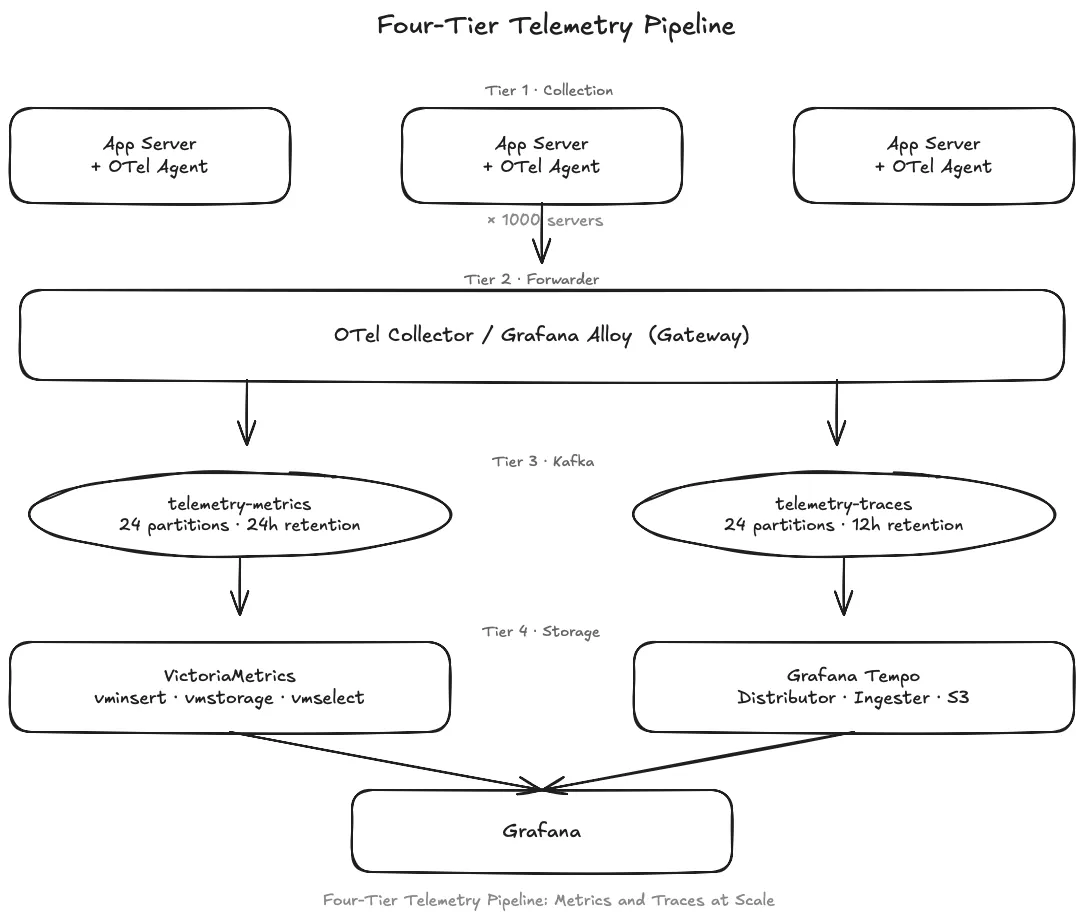
4. The Architecture: Four Tiers, One Job Each#
Each tier has exactly one job, and those jobs do not overlap:
- Tier 1 — Agents run on every server. They collect from all local sources and push raw telemetry upstream. Nothing is filtered, enriched, or sampled at this layer.
- Tier 2 — Forwarders run on dedicated machines and handle all processing: filtering noise, enriching attributes, running tail sampling on traces, converting spans to span metrics, and batching for Kafka.
- Tier 3 — Kafka absorbs the full write rate from all forwarders and decouples processing from storage. When VictoriaMetrics is upgrading or Tempo is slow, forwarders keep writing to Kafka without backing up into the agents.
- Tier 4 — Consumers read from Kafka at the pace storage can absorb and write to the appropriate backend — VictoriaMetrics for metrics, Grafana Tempo for traces.
Two rules hold the design together:
Agents do not process. All work that can be deferred — filtering, relabeling, enrichment, sampling — moves to dedicated forwarder machines. This keeps agent memory under 500 MB on every production server regardless of fleet size.
Kafka is the boundary, not just a buffer. Forwarders write to Kafka and return immediately. Consumers pull at their own pace. Storage pressure, rolling upgrades, and temporary slowdowns never reach the agents or the applications they run alongside.
5. Tier 1 — The Agent: Collect Everything, Process Nothing#
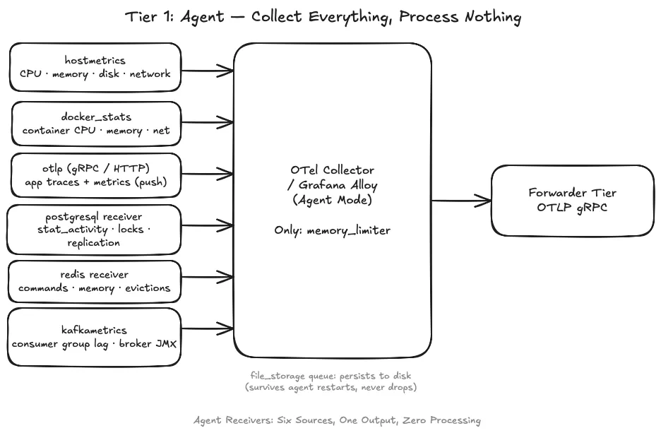
The agent runs on every server. Its only job is to receive telemetry from all local sources and forward it upstream. Nothing else.
OpenTelemetry Collector vs Grafana Alloy#
Both are valid choices. They share the same receiver ecosystem and both speak OTLP natively.
OpenTelemetry Collector is vendor-neutral, uses YAML, and has the broadest community support. Use it if you want portability or are already using the OTel ecosystem.
Grafana Alloy is Grafana’s distribution of the OTel Collector. It uses the River/Alloy config language and integrates more closely with the Grafana stack. If you already use Grafana for dashboards and alerts, Alloy can be easier to manage at larger scale.
The underlying pipeline behavior is identical. Configs for both — OTel YAML and Alloy River — are in the companion repository.
What the Agent Collects#
Every server runs one agent. The same base receivers run everywhere; service-specific receivers layer on top based on the server’s role.
Base — every server:
hostmetrics— CPU, memory, disk I/O, network throughput, filesystem usage, running processes. This is the foundation regardless of what the server runs.otlp— a receiver, not a scraper. Instrumented services push their traces and custom metrics to the agent on port 4317 (gRPC) or 4318 (HTTP). This is how application spans enter the pipeline — services push to the local agent, not to a central endpoint.
Runtime — choose one based on how workloads are deployed:
-
Docker:
docker_stats— per-container CPU, memory, network, and block I/O from the Docker stats API, without cAdvisor overhead. Series count scales with container density — 100 containers on a 16-core server with several NICs generates roughly 8,000 series (per-core CPU, per-interface network, per-device block I/O). -
Kubernetes worker node:
kubeletstats— node, pod, and container metrics from the kubelet API on the local node. Key signals it gives you:k8s.node.cpu.usage,k8s.node.memory.working_set— actual node consumption, not requests or limitsk8s.pod.cpu.usage,k8s.pod.memory.working_set— per-pod actual usage; the gap between this and the pod’s memory limit is your headroom before OOMKillk8s.container.cpu.request.utilization,k8s.container.memory.request.utilization— how close a container is to its resource request, the primary signal for right-sizingk8s.pod.network.io,k8s.pod.network.errors— pod-level I/O without needing a CNI plugin- Auth:
auth_type: serviceAccountagainst the local node’s kubelet. No cluster-wide permissions required.
-
Kubernetes cluster state:
k8s_cluster— the control-plane view of resource object states. Run one dedicated collector per cluster, not per worker node. Key signals:k8s.deployment.desiredvsk8s.deployment.available— the gap is pods that failed to startk8s.pod.phaseby phase (Pending, Running, Failed, Succeeded, Unknown) — fastest cluster-wide pod health signalk8s.node.conditionby type (Ready, MemoryPressure, DiskPressure, PIDPressure) — node health that drives scheduling decisionsk8s.hpa.desired_replicasvsk8s.hpa.current_replicas— whether autoscaling is catching up or stuck
-
Kubernetes events:
k8sevents— collects the Kubernetes API event stream. Not metrics, but some of the highest-signal data in the cluster for correlating spikes with what actually changed. Key event reasons:OOMKilled— container exceeded its memory limit; always warrants investigationBackOff/CrashLoopBackOff— a pod that cannot start; usually a config or dependency problemFailedScheduling— no node can fit the pod; cluster is at capacity or constraints are too tightEvicted— kubelet evicted a pod due to node memory or disk pressureSuccessfulRescale— HPA scaled a deployment; correlate with traffic spikes- Note:
k8seventsemits logs, not metrics. It needs a separate logs pipeline (Loki or VictoriaLogs) — out of scope for this post. Run one dedicated collector per cluster, not on every worker node.
Services — enable per role:
- Databases (
postgresql,mysql,mongodb) at 60s — query throughput, connections, replication lag, buffer pool stats. 60 seconds matters: scraping more often adds measurable load to a busy primary. - Caches (
redis) at 15s — eviction rate, hit/miss ratio. Eviction rate can spike and recover within a single scrape window, so 15 seconds is worth it. - Brokers (
kafkametrics) at 30s — consumer group lag by topic and partition, the clearest signal for whether your event-driven system is keeping up. - Web and proxy (
nginx,haproxy) — active connections, request rates, error rates.
Traces and spans:
Application traces arrive via otlp alongside metrics. Instrumented services push spans to the agent on localhost:4317 (gRPC) or localhost:4318 (HTTP/proto). The agent forwards everything unmodified — no sampling at this tier.
A trace is a tree of spans, one per unit of work across a distributed request. Each span carries:
| Field | What It Contains |
|---|---|
trace_id | 128-bit ID shared across every span in one request |
span_id | 64-bit ID for this specific operation |
parent_span_id | Links to the span that called this one; nil on the root span |
name | Operation label: GET /api/users, SELECT users, kafka.produce |
start_time / end_time | Nanosecond-precision timestamps |
status | OK, ERROR, or UNSET |
attributes | Key-value pairs following OTel semantic conventions |
events | Time-stamped annotations within the span: exceptions, retries, checkpoints |
links | References to spans in other traces — used in async and message-driven flows |
The attributes follow OTel semantic conventions — standard names across all SDKs and languages:
# HTTP service span
http.method = "GET"
http.route = "/api/users/{id}"
http.response.status_code = 200
server.address = "api.example.com"

# Database call span
db.system = "postgresql"
db.name = "users_db"
db.statement = "SELECT id, email FROM users WHERE id = $1"
db.operation.name = "SELECT"
server.address = "postgres-primary.internal"
OTel SDKs for Go, Python, Java, Node.js, and .NET auto-instrument HTTP clients/servers, gRPC, database drivers, and message queue clients with no code changes. Manual instrumentation adds business-level spans — checkout.validate, payment.authorize, inventory.reserve — that libraries cannot infer.
The One Rule: Collect and Forward, Nothing Else#
The agent runs exactly one processor: memory_limiter. That is the complete list.
No filtering — all metrics forward upstream. Noise is dropped at the forwarder, not here.
No enrichment — no env labels, no region tags. Adding them at the agent means touching every server’s config when labels change.
No sampling — every span forwards. Tail sampling at the forwarder needs the full trace to make decisions.
The pipeline wiring reflects this:
service:
  pipelines:
    metrics:
      receivers:  [hostmetrics, docker_stats, otlp, postgresql, redis]  # adjust per role
      processors: [memory_limiter]   # the only processor at this tier
      exporters:  [otlp]             # always the forwarder, never storage directly
    traces:
      receivers:  [otlp]
      processors: [memory_limiter]
      exporters:  [otlp]
Everything flows to the forwarder over OTLP gRPC. The agent never writes to VictoriaMetrics, Tempo, or Kafka directly.
Receivers Worth Adding First#
Database and middleware receivers often give the most value for the least setup work. A few stand out:
PostgreSQL receiver gives you pg_stat_activity (active connections, query states, wait events), table bloat estimates, replication lag, and lock contention. These are much more useful than disk-level metrics alone. Set collection_interval: 60s so you do not add noticeable load to a busy primary.
Redis receiver exposes redis.keys.evicted, which is often the most important Redis metric. A non-zero eviction rate means your keyspace is larger than available memory and cached data is being dropped. You cannot see that from node-level memory metrics alone.
Kafka metrics receiver gives you consumer group lag by topic and partition. This is often the clearest sign of whether your event-driven system is keeping up. If lag keeps growing, something downstream is falling behind.
MySQL receiver surfaces InnoDB buffer pool efficiency, slow query counts, and replication delay in one pass. These metrics are hard to collect cleanly without a purpose-built receiver.
Prometheus receiver (prometheus) — scrapes any /metrics endpoint in Prometheus exposition format. This covers anything that has not switched to OTel natively: Node Exporter, custom app metrics, third-party exporters. It is a drop-in replacement for Prometheus scraping without running Prometheus itself.
receivers:
  prometheus:
    config:
      scrape_configs:
        - job_name: app-custom-metrics
          scrape_interval: 15s
          static_configs:
- targets: ["localhost:9090"]6. Tier 2 — The Forwarder: The Brain of the Pipeline#
The forwarder runs on dedicated machines, not on your app servers. Each forwarder handles 50 to 100 agent connections at high volume. This is where all the work that the agent deliberately avoided now happens.
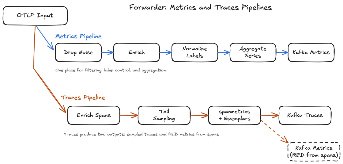
The forwarder runs two independent pipelines inside the same collector process: one for metrics, one for traces. They use different processors, different exporters, and write to different Kafka topics.
Metrics Pipeline: Four Steps in Order#
Step 1 — Drop noise. Filter metrics that will never be queried. Dropping here means less data in Kafka, less in storage, and faster queries. The agent forwards everything; the forwarder decides what matters. The main categories to drop:
- Go runtime internals (
process.runtime.go.gc.*): useful in profiling sessions, not in dashboards. - Individual HTTP endpoint metrics: too much cardinality. Status class (2xx, 4xx, 5xx) is sufficient for alerting.
- Elasticsearch index-level metrics: 500 indices means 500x your series count. Enable only for indices you actively monitor.
- Container labels as metric dimensions: keep only team, service, and environment. Docker and Kubernetes generate dozens of labels per container — forwarding them multiplies series count without adding alerting value.
- Collector self-telemetry (
otelcol_*): route this to a separate internal observability pipeline, not to the main metrics topic.
processors:
  filter/drop_noise:
    metrics:
      exclude:
        match_type: regexp
        metric_names:
          - "process\\.runtime\\.go\\..*"   # Go GC internals — useful in profiling, not in dashboards
          - "otelcol_.*"                     # collector self-telemetry — goes to a separate ops pipeline
          - "container_tasks_state"          # container lifecycle counter, not useful for alerting
          - ".*\\.scrape_duration_seconds"   # scrape overhead, not a service metric
Step 2 — Enrich.
Add infrastructure labels: deployment.environment, cloud.region, k8s.cluster.name, team. This is the single place in the entire pipeline where these labels are added. One config change here propagates to every metric from every server. This is what makes enrichment at the agent impractical — you would need to update and redeploy a thousand agent configs to change a label.
processors:
  attributes/enrich:
    actions:
      - {key: deployment.environment, value: production,      action: upsert}
      - {key: cloud.region,           value: us-east-1,       action: upsert}
      - {key: k8s.cluster.name,       value: prod-cluster-1,  action: upsert}
      - {key: team,  from_attribute: service.namespace,       action: upsert}
The from_attribute form copies a value that the agent already attached — the agent sets service.namespace from the local environment variable at startup, the forwarder promotes it into the team label. No label hardcoded at the agent.
Step 3 — Normalize. Standardize metric names and collapse high-cardinality label values. HTTP status codes (200, 201, 204, 400, 404, 500…) become status classes (2xx, 4xx, 5xx). Metric names from different instrumentation libraries get unified to OTel semantic conventions. High-cardinality histograms get aggregated down to the label dimensions that matter for alerting. This step is what makes 12M series manageable at query time.
The most common cardinality explosion is HTTP status codes. Every unique status code value is a separate series. Collapsing to three classes (2xx, 4xx, 5xx) reduces the series count by a factor equal to the number of distinct codes your services emit.
processors:
  transform/normalize:
    metric_statements:
      - context: datapoint
        statements:
          # Collapse HTTP status code → status class. One label, three values instead of hundreds.
          - set(attributes["http.status_class"], "2xx") where IsMatch(attributes["http.status_code"], "2\\d\\d")
          - set(attributes["http.status_class"], "4xx") where IsMatch(attributes["http.status_code"], "4\\d\\d")
          - set(attributes["http.status_class"], "5xx") where IsMatch(attributes["http.status_code"], "5\\d\\d")
          - delete_key(attributes, "http.status_code") where attributes["http.status_class"] != nil
          # Drop per-pod identifiers that make series unique but carry no alerting value
          - delete_key(attributes, "net.host.name")
          - delete_key(attributes, "http.target")
delete_key on net.host.name is the most impactful single rule. Individual pod hostnames make every pod a unique series. Removing the hostname and keeping k8s.pod.name only where it matters cuts series by a factor equal to replica count.
Step 4 — Batch and write to Kafka.
Metrics land in the telemetry-metrics topic as otlp_proto (binary, not JSON — roughly 30–40% smaller). required_acks: -1 means all in-sync replicas acknowledge before the write is confirmed. snappy compression. The forwarder never writes directly to VictoriaMetrics.
service:
  pipelines:
    metrics:
      receivers:  [otlp]
      processors: [memory_limiter, filter/drop_noise, attributes/enrich,
                   transform/normalize, metricstransform/aggregate, batch]
      exporters:  [kafka/metrics]
Traces Pipeline: Three Steps the Metrics Pipeline Does Not Have#
Enrich spans. Same label set as metrics — environment, region, cluster name. Every span gets the same infrastructure context as the host metrics from the same server.
Tail sampling. This is the core reason the forwarder tier exists in this design. Four policies run in priority order:
- Keep 100% of error traces. Any trace where at least one span has ERROR status is kept unconditionally. During an incident, you need every failed request, not a 20% sample of them.
- Keep 100% of slow traces. Any trace where end-to-end latency exceeded 2 seconds is kept. Slow requests are the ones you investigate — sampling them away defeats the purpose.
- Keep 100% of critical services. Payment, checkout, and order flows are kept regardless of outcome. The business cost of losing a trace here is higher than the storage cost of keeping it.
- Keep 20% of everything else. Normal, fast, successful traffic is sampled probabilistically. This is where the 3M spans/sec becomes 500K after sampling.
The decision_wait is 30 seconds — the forwarder holds spans in memory for up to 30 seconds before making a keep-or-drop decision. This is why tail sampling requires dedicated machines with sufficient RAM, and why every span of a trace must reach the same forwarder instance. The load balancer in front of the forwarder pool must use consistent hashing on trace ID. A round-robin load balancer splits traces across instances and makes tail sampling effectively random.
processors:
  tail_sampling:
    decision_wait: 30s
    num_traces: 500000              # max traces held in memory simultaneously — size this generously
    expected_new_traces_per_sec: 10000
    policies:
      - name: keep-errors           # 100% — any span with ERROR status keeps the whole trace
        type: status_code
        status_code: {status_codes: [ERROR]}
      - name: keep-slow             # 100% — traces slower than 2s are kept unconditionally
        type: latency
        latency: {threshold_ms: 2000}
      - name: keep-critical-services  # 100% — business-critical flows, always keep
        type: string_attribute
        string_attribute:
          key: service.name
          values: [payment-service, checkout-service, order-service]
      - name: probabilistic-sample  # 20% of everything else
        type: probabilistic
        probabilistic: {sampling_percentage: 20}
num_traces is the number of in-flight traces the forwarder holds in memory simultaneously. At 10,000 new traces/sec and a 30-second window, you need at least 300,000 slots — 500,000 leaves room for traffic spikes without OOMing the forwarder. The formula is expected_new_traces_per_sec × decision_wait_seconds × safety_factor. See the companion repository for per-instance memory sizing.
Span metrics.
Before traces are sampled, the spanmetrics connector generates RED metrics (request rate, error rate, duration histograms) from the raw span data. These go to the telemetry-metrics Kafka topic — not the traces topic. This means your latency dashboards and error rate alerts are based on 100% of request traffic, even though only 20% of normal traces make it to Tempo.
spanmetrics is a connector in the OTel model: it receives all incoming spans (before the tail sampling decision) in a dedicated pipeline and emits the RED metrics into a separate metrics pipeline. The tail sampling pipeline runs independently on the same span stream. Two pipelines, same incoming otlp receiver — the OTel Collector fans the data out internally.
service:
  pipelines:
    traces/spanmetrics:              # sees 100% of spans — generates RED metrics before any sampling
      receivers:  [otlp]
      processors: [memory_limiter, attributes/enrich_spans]
      exporters:  [spanmetrics]      # spanmetrics is a connector, not a processor
    traces/sampled:                  # tail-samples the same incoming spans independently
      receivers:  [otlp]
      processors: [memory_limiter, tail_sampling, batch/traces]
      exporters:  [kafka/traces]
    metrics/from_spans:              # RED metrics generated by the spanmetrics connector
      receivers:  [spanmetrics]
      processors: [batch]
      exporters:  [kafka/metrics]    # same Kafka topic as the metrics pipeline
Full forwarder configs — all OTTL transform statements, Kafka producer settings, spanmetrics histogram buckets and dimensions — are in the companion repository.
Part 2: Making It Durable at Scale#
At this point, the collection path is in place. Agents stay lightweight on production machines, and forwarders become the single place for enrichment, normalization, sampling, and span-to-metrics conversion.
What remains is the hardening work that turns a good architecture into a reliable one: deterministic trace routing, Kafka buffering, storage backends, dashboards, sizing, and failure handling.
That is the focus of Part 2: tail sampling, cardinality control, Kafka, VictoriaMetrics, Grafana Tempo, capacity planning, and production HA.