Designing a Telemetry Pipeline That Scales [Part 2]: Sampling, Kafka, Storage, and HA
How to make the pipeline durable at scale with tail sampling, Kafka buffering, VictoriaMetrics, Tempo, and production hardening.
This is Part 2 of a two-part series on building a telemetry pipeline for 1,000 servers. Part 1 covered the collection path: where common designs break, how to split the system into clear tiers, and why agents and forwarders should have very different jobs.
At that point, the collection path was in place. Agents stayed lightweight on production machines, and forwarders became the single place for enrichment, normalization, sampling, and span-to-metrics conversion.
What remained was the hard part: making the pipeline correct, durable, and easy to operate under real load.
This post covers that half of the design: tail sampling, cardinality control, Kafka buffering, storage backends, capacity planning, and high availability.
7. Tail Sampling: Why Head Sampling Fails at Scale#
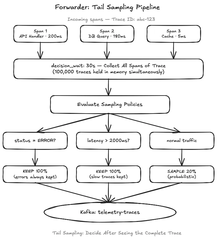
Tail sampling buffers all spans of a trace for up to 30 seconds and evaluates policies against the complete picture — unlike head sampling, which flips a coin before the request finishes and can drop the one slow database query that caused the incident while retaining 10,000 uneventful traces.
Request arrives and generates Trace ID: 7a3f-c91b

  Span 1:  api-gateway     (12ms)
  Span 2:  user-service    (8ms)
  Span 3:  postgres-query  (1,850ms)   <- 1.85 seconds, slow
  Span 4:  cache-lookup    (2ms)

  Total trace duration: 1,872ms

Tail sampling evaluation:
  keep-slow-traces threshold is 2000ms  -> not triggered at 1,872ms
  keep-errors: no ERROR status spans    -> not triggered
  sample-normal-traffic: 20% random    -> keep or drop by chance

Recommendation: tune the latency threshold to your SLO, not a round number.
Set threshold_ms: 1500 and you catch this trace every time.
The Consistent Routing Requirement#
Tail sampling has one hard constraint: all spans of the same trace must arrive at the same forwarder instance. If Span 1 goes to forwarder-A and Span 2 goes to forwarder-B, neither instance has enough information to make a sampling decision.
The fix is consistent hashing at the load balancer layer. Hashing on the traceparent or X-B3-TraceId header guarantees that all spans sharing a trace ID land on the same forwarder.
If you are chaining OTel collectors, the loadbalancingexporter handles this automatically:
exporters:
  loadbalancing:
    protocol:
      otlp:
        tls:
          insecure: true
    resolver:
      static:
        hostnames:
          - forwarder-1:4317
          - forwarder-2:4317
          - forwarder-3:4317
    routing_key: traceID # consistent hash on trace ID
Memory Sizing for Tail Sampling#
num_traces sets the maximum concurrent traces in memory. At 10,000 new traces per second and a 30-second decision_wait, the buffer needs at least 300,000 slots — set it to 500,000 to absorb traffic spikes without the forwarder evicting traces before their window closes. Monitor otelcol_processor_tail_sampling_count_traces_sampled_late. Any non-zero value means spans arrived after the sampling decision was already made, which means the buffer is undersized or decision_wait is too short.
At 8 to 16GB RAM per forwarder, you can comfortably hold 200,000 to 400,000 concurrent traces at roughly 40KB per trace in memory.
8. spanmetrics: RED Metrics from Traces for Free#
The spanmetrics connector generates service-level metrics directly from your trace spans. No additional instrumentation is required, and no changes to your applications are needed.
From your existing traces, it produces:
| Metric | What It Measures |
|---|---|
calls_total | Request rate per service, endpoint, and status |
duration_milliseconds_bucket | Latency histogram enabling p50, p95, p99 calculations |
duration_milliseconds_sum | Cumulative total latency |
duration_milliseconds_count | Total request count |
These are your RED metrics (Rate, Errors, Duration), the standard service health signals, generated automatically from the traces your apps already emit.
The critical feature is exemplars. When spanmetrics is configured with exemplars.enabled: true, each metric data point carries a reference to an actual trace ID. In Grafana, you can click from a p99 latency spike directly into the trace that caused it, with no manual correlation required.
connectors:
  spanmetrics:
    # Fewer dimensions = fewer series. These four cover most alerting needs.
    dimensions:
      - name: http.method # GET, POST, etc.
      - name: http.status_class # 2xx, 4xx, 5xx — set by transform/normalize, not the raw code
      - name: deployment.environment
      - name: rpc.service # downstream service name for dependency graphs
    exemplars:
      enabled: true # attaches a trace ID to each data point for Grafana click-through
The generated metrics feed directly into the kafka/metrics exporter alongside your regular metrics, flowing through the same pipeline into VictoriaMetrics. They appear in Grafana like any other metric.
9. Cardinality: The Silent Pipeline Killer#
Cardinality is the number of unique label value combinations for a metric. A metric http_requests_total with labels for method, status code, and endpoint has cardinality equal to the number of methods multiplied by the number of status codes multiplied by the number of unique endpoints.
At 1,000 endpoints with GET and POST across five status codes, that is 10,000 series for one metric. Add a user_id or request_id label and it becomes 10,000 multiplied by the number of unique users, resulting in millions of series for a single metric.
VictoriaMetrics handles high cardinality significantly better than Prometheus, but no storage system survives unbounded growth indefinitely.
Where Cardinality Explodes#
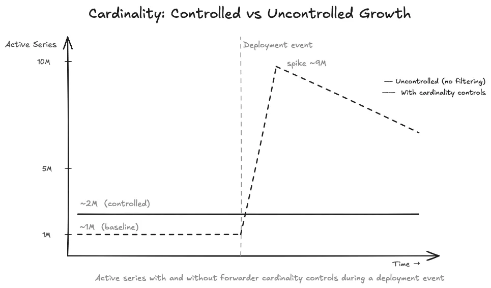
Deployments create new pod names, new IPs, and new replica IDs. If any of those values are metric label dimensions, every deployment creates a new series for every existing metric. Old series go stale but count against your active series total until they expire.
High-cardinality label values such as user IDs, request IDs, session tokens, and trace IDs in metric labels are cardinality bombs. Any label with unbounded unique values grows without limit.
Container labels forwarded as metric dimensions. Docker and Kubernetes generate dozens of labels per container. Forwarding those through as metric dimensions creates label spaces that are impossible to manage.
The Fix: Transform at the Forwarder#
The transform/normalize processor handles this at the forwarder tier — collapsing HTTP status codes to 2xx/4xx/5xx and dropping pod-specific labels like k8s.pod.name and container.id that make every replica a unique series. That config is covered in the Part 1 forwarder section.
The second processor, metricstransform/aggregate, handles deployment-related cardinality by reducing histograms to a fixed label set:
processors:
  metricstransform/aggregate:
    transforms:
      - include: http.server.request.duration
        action: update
        operations:
          - action: aggregate_labels
            # Only these four dimensions reach VictoriaMetrics — everything else is dropped
            label_set: [deployment.environment, k8s.cluster.name, http.method, http.status_class]
            aggregation_type: sum
The practical result: a deployment that would have created 500,000 new series (one per pod multiplied by endpoint count) creates zero new series. The active series count stays flat through rolling deploys.
10. Tier 3 — Kafka: Decoupling That Saves Your Storage#
Kafka sits between the forwarder and storage. At this scale it is not optional. It is the buffer that prevents a 10-minute VictoriaMetrics upgrade from creating a 10-minute gap in your metrics.
Two Topics, Different Characteristics#
Topic: telemetry-metrics
  Partitions:         24
  Replication Factor: 3
  Retention:          24 hours
  Partition key:      hash(metric_name + labels)
  Compression:        snappy

Topic: telemetry-traces
  Partitions:         24
  Replication Factor: 3
  Retention:          12 hours  (traces are larger; shorter retention is fine)
  Partition key:      trace_id  (all spans of a trace land in the same partition)
  Compression:        snappy
Metrics and traces get separate topics because their consumption patterns differ fundamentally. Metrics require ordering within a series for correct rate calculations. Traces require grouping by trace ID for correlated queries. Separate topics mean separate consumer groups, independent offsets, and the ability to scale each consumer independently without affecting the other.
Kafka Broker Configuration#
# Replication safety
default.replication.factor=3
min.insync.replicas=2
unclean.leader.election.enable=false

# Performance
num.io.threads=16
num.network.threads=8
num.replica.fetchers=4
socket.send.buffer.bytes=1048576
socket.receive.buffer.bytes=1048576

# Retention
log.retention.hours=24
log.retention.bytes=107374182400    # 100GB per partition max
log.segment.bytes=1073741824        # 1GB segments

# Compression
compression.type=snappy
Setting min.insync.replicas=2 with RF=3 means a write is only acknowledged after two of three replicas confirm it. You can lose one broker with no data loss. Setting unclean.leader.election.enable=false ensures a broker that has fallen behind in replication never becomes the partition leader and does not discard committed messages during the transition.
11. Tier 4a — VictoriaMetrics: Storing Millions of Series#
VictoriaMetrics handles metrics storage. The cluster mode provides HA and horizontal scaling.
The cluster has three component types:
- vminsert receives writes and distributes them across vmstorage nodes.
- vmstorage stores the actual time series data, sharded by metric name.
- vmselect handles queries and merges results from all vmstorage nodes.
vminsert flags:
  --storageNode=vmstorage-1:8400
  --storageNode=vmstorage-2:8400
  --storageNode=vmstorage-3:8400
  --replicationFactor=2

vmstorage flags:
  --retentionPeriod=15d
  --downsampling.period=30d:5m    # after 30 days, keep 5-minute resolution
  --downsampling.period=90d:1h    # after 90 days, keep 1-hour resolution
  --maxConcurrentInserts=64
Downsampling is critical for long-term retention. Raw 15-second data is only useful for recent incidents. For week-over-week trends and capacity planning, 5-minute resolution is more than sufficient and uses 20 times less storage. With the config above, a 6-month retention period uses roughly the same storage as 30 days of raw data.
Metrics Consumer Config#
The consumer reads from the Kafka telemetry-metrics topic and writes to VictoriaMetrics via Prometheus remote write:
receivers:
  kafka/metrics:
    brokers: [kafka1:9092, kafka2:9092, kafka3:9092]
    topic: telemetry-metrics
    encoding: otlp_proto
    group_id: victoriametrics-consumer # isolated offset tracking from traces consumer

exporters:
  prometheusremotewrite:
    endpoint: http://vminsert:8480/insert/0/prometheus/api/v1/write
    resource_to_telemetry_conversion:
      enabled: true # convert OTel resource attributes to Prometheus labels
    retry_on_failure:
      enabled: true
      max_elapsed_time: 0 # retry forever — Kafka holds the backlog during outages

service:
  pipelines:
    metrics:
      receivers: [kafka/metrics]
      processors: [memory_limiter, batch]
      exporters: [prometheusremotewrite]
12. Tier 4b — Grafana Tempo: Storing Billions of Spans#
Tempo stores traces in object storage. This is the correct model for trace data: traces are large, written once, and mostly accessed during incident debugging rather than aggregate analysis. The absence of an intermediate storage system (like Cassandra) is the key difference from Jaeger.
server:
  http_listen_port: 3200

distributor:
  receivers:
    otlp:
      protocols:
        grpc:
          endpoint: 0.0.0.0:4317

storage:
  trace:
    backend: s3
    s3:
      bucket: telemetry-traces-prod
      endpoint: s3.amazonaws.com
      region: us-east-1
    wal:
      path: /var/tempo/wal # write-ahead log on local disk
    pool:
      max_workers: 100
      queue_depth: 10000

compactor:
  compaction:
block_retention: 336h # 14 daysTraces Consumer Config#
receivers:
  kafka/traces:
    brokers: [kafka1:9092, kafka2:9092, kafka3:9092]
    topic: telemetry-traces
    encoding: otlp_proto
    group_id: tempo-consumer # isolated offset tracking from metrics consumer

exporters:
  otlp/tempo:
    endpoint: http://tempo-distributor:4317
    tls:
      insecure: true
    retry_on_failure:
      enabled: true
      max_elapsed_time: 0 # retry forever — Kafka holds the backlog during outages

service:
  pipelines:
    traces:
      receivers: [kafka/traces]
      processors: [memory_limiter, batch]
      exporters: [otlp/tempo]
13. Grafana: Wiring It All Together#
Grafana connects to both storage backends and provides a unified view across metrics and traces.
apiVersion: 1
datasources:
  - name: VictoriaMetrics
    type: prometheus
    url: http://vmselect:8481/select/0/prometheus
    isDefault: true
    jsonData:
      timeInterval: '15s'

  - name: Grafana Tempo
    type: tempo
    url: http://tempo:3200
    jsonData:
      tracesToMetrics:
        datasourceUid: victoriametrics
        tags:
          - key: service.name
            value: service
          - key: rpc.service
      serviceMap:
        datasourceUid: victoriametrics
      nodeGraph:
        enabled: true
      search:
        hide: false
      lokiSearch:
        datasourceUid: loki
The tracesToMetrics configuration links trace spans to the RED metrics generated by spanmetrics. When you are viewing a specific trace in Tempo, you can click through to see the corresponding metrics for that service at that exact timestamp. The link also works in reverse: Grafana metric dashboards with exemplars enabled let you click from a p99 latency data point directly into the trace that produced it.
Key Dashboards to Build First#
- Pipeline health: agent queue depth, forwarder memory usage, Kafka consumer group lag, VictoriaMetrics ingestion rate, Tempo distributor spans received.
- Service RED metrics: rate, error rate, and duration per service from spanmetrics, with exemplar links to traces for click-through debugging.
- Infrastructure overview: CPU, memory, and disk per server role (app servers, database servers, Kafka brokers).
- Cardinality watch: active series count in VictoriaMetrics, series growth rate over time, top series by label combination.
14. Capacity Planning: Numbers Before You Build#
Size each tier before deploying. Surprises in infrastructure sizing are expensive to fix after the fact.
Collection Tier (Agents)#
Per agent:
  CPU:   0.3 to 0.5 cores at steady state
  RAM:   400 to 600MB (memory_limiter caps at 400MB plus OS overhead)
  Disk:  5 to 20GB for file_storage queue
  Scale: 1 per server, deployed as a systemd service or Kubernetes DaemonSet
Forwarder Tier#
Per forwarder:
  CPU:   4 to 8 cores (tail_sampling is the CPU-intensive step)
  RAM:   8 to 16GB (tail_sampling buffers 200k to 400k traces; size num_traces accordingly)
  Scale: 1 forwarder per 50 to 100 agent connections

For 1,000 servers:
  10 to 20 forwarder instances
  Consistent-hash load balancer in front (required for tail sampling)
Kafka Cluster#
Throughput:
  Metrics: ~500MB/s raw, 60MB/s compressed (snappy achieves ~8:1 on metrics proto)
  Traces:  ~3M spans/sec x 1KB average = 3GB/s raw, 600MB/s compressed

Storage per day:
  Metrics: 60MB/s x 86,400s x 3 replicas = ~15TB
  Traces:  600MB/s x 43,200s x 3 replicas = ~75TB (12-hour retention)

Recommendation:
  6 brokers x 20TB NVMe each
25Gbit networking (traces are bandwidth-intensive)VictoriaMetrics#
RAM: approximately 1GB per 1M active series
  5M active series needs 5 to 8GB RAM per vmstorage node with headroom

Storage (15d raw plus downsampled):
  Raw 15 days:        ~13TB
  With downsampling:  ~16TB total

Recommendation:
  3 vmstorage nodes, 6TB SSD each
  2 vminsert and 2 vmselect (both stateless, easy to scale)
Grafana Tempo#
Trace storage (post-sampling, 14-day retention):
  300,000 spans/sec x 1KB x 86,400s x 14 days = ~360TB uncompressed
  With 10:1 snappy compression on S3           = ~36TB on S3

S3 cost at $0.023/GB/month: approximately $830/month for 14 days of trace data15. Production Hardening: HA, Queuing, and Backpressure#
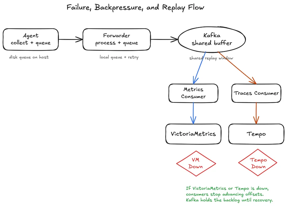
Every tier in this pipeline is designed to queue when its downstream is unavailable and replay when that downstream recovers. No data is lost as long as recovery happens within the queue retention window.
Failure Modes by Tier#
| Tier Failure | Impact | Recovery |
|---|---|---|
| Single agent crash | Gap in that server’s telemetry only | Agent restarts; file_storage queue replays from last position |
| Agent to forwarder network loss | Agent queues to disk until network recovers | Replays from disk queue; no data lost |
| Forwarder crash | Agents queue to disk for hours of capacity | Forwarder restarts; agents drain their queues |
| Single Kafka broker | Transparent with RF=3 and ISR=2 | Leader election completes in approximately 30 seconds |
| All Kafka brokers down | Forwarders queue to disk with max_elapsed_time: 0 | Kafka recovers; forwarders drain automatically |
| VictoriaMetrics down | Metrics consumer falls behind in Kafka (24-hour retention) | VM recovers; consumer catches up from its saved offset |
| Grafana Tempo down | Traces consumer falls behind in Kafka (12-hour retention) | Tempo recovers; consumer catches up from its saved offset |
| Single vmstorage node lost | replicationFactor=2 absorbs the loss transparently | Rebalances when the node returns |
Pipeline Self-Monitoring#
# Alert rules for the pipeline itself

groups:
  - name: telemetry-pipeline
    rules:
      # Agent queue building: forwarder may be unreachable
      - alert: AgentQueueDepthHigh
        expr: otelcol_exporter_queue_size{exporter="otlp"} > 5000
        for: 5m

      # Tail sampling making late decisions: buffer may be undersized
      - alert: TailSamplingLateSamples
        expr: increase(otelcol_processor_tail_sampling_count_traces_sampled_late[5m]) > 0

      # Kafka consumer falling behind: storage may be slow or unavailable
      - alert: MetricsConsumerLagHigh
        expr: kafka_consumer_group_lag{group="victoriametrics-consumer"} > 100000

      - alert: TracesConsumerLagHigh
        expr: kafka_consumer_group_lag{group="tempo-consumer"} > 50000

      # VictoriaMetrics cardinality approaching limits
      - alert: CardinalityHigh
        expr: vm_active_time_series > 10000000

      # VictoriaMetrics storage under pressure
      - alert: VMSlowInserts
        expr: rate(vm_slow_row_inserts_total[5m]) > 0
High-Availability Deployment#
Forwarder tier: Run three or more forwarder instances behind a consistent-hash load balancer. The load balancer must use trace ID as the hash key. If it does not, spans from the same trace land on different forwarder instances and tail sampling cannot function.
Kafka: Three brokers minimum with RF=3 and min.insync.replicas=2. Use either a dedicated ZooKeeper ensemble or KRaft mode (Kafka 3.x and later). Place brokers in separate availability zones.
VictoriaMetrics: Setting --replicationFactor=2 on vminsert ensures every metric write goes to two vmstorage nodes. Run two or more vminsert and vmselect instances since both are stateless. Run three or more vmstorage nodes.
Grafana Tempo: Run two or more distributor and ingester instances. Ingesters are stateful and use a memberlist ring for coordination. The compactor runs as a single instance since it only processes completed blocks already in object storage.
16. What’s Next: The Intelligence Layer#
This post covered the infrastructure: how to move telemetry from 1,000 servers to storage reliably at millions of events per second. The pipeline handles collection, processing, buffering, and storage.
What it does not do is help you understand what you are seeing.
A follow-up post covers the intelligence layer built on top of this pipeline:
Flink correlation engine: a streaming job that consumes from both Kafka topics simultaneously, correlates metric anomalies with trace patterns, and publishes correlated events to a dedicated Kafka topic (grafana-webhook-alert-correlations-v1). When an alert fires, the correlation engine already has the matching traces and related metric patterns ready.
Alert correlation: Grafana alerts publish to the correlation topic. The Flink job enriches each alert with related services from trace service graphs, correlated metric anomalies from the metrics stream, and similar past incidents from the event history.
HolmesGPT SRE agent: an AI agent connected to VictoriaMetrics, the log pipeline, and the correlation topic. When an alert fires, HolmesGPT queries the relevant metrics and retrieves correlated traces to produce a starting point for investigation — significantly reducing initial triage time.
ClickHouse for correlated event storage: Flink output lands in ClickHouse, which handles the analytical query patterns (time range scans and multi-signal correlations) that neither VictoriaMetrics nor Tempo are optimized for.
The infrastructure in this post is the prerequisite. Without reliable and complete telemetry flowing from every server into storage, the intelligence layer has nothing to work with.